
age int64 | status int64 | sex int64 | orientation int64 | body_type int64 | diet int64 | drinks int64 | drugs int64 | education int64 | ethnicity int64 | height float64 | income int64 | job int64 | location int64 | pets int64 | religion int64 | sign int64 | smokes int64 | days_since_online int64 | num_languages float64 |
|---|---|---|---|---|---|---|---|---|---|---|---|---|---|---|---|---|---|---|---|
22 | 3 | 1 | 2 | 0 | 0 | 4 | 0 | 3 | 0 | 75 | 43,840 | 19 | 1 | 14 | 0 | 4 | 1 | 2 | 1 |
35 | 3 | 1 | 2 | 2 | 3 | 2 | 2 | 3 | 8 | 70 | 80,000 | 8 | 1 | 14 | 0 | 2 | 0 | 1 | 3 |
38 | 0 | 1 | 2 | 10 | 0 | 4 | 1 | 4 | 5 | 68 | 181,707 | 8 | 1 | 5 | 2 | 7 | 0 | 3 | 3 |
23 | 3 | 1 | 2 | 10 | 5 | 4 | 0 | 3 | 8 | 71 | 20,000 | 18 | 1 | 10 | 2 | 7 | 0 | 2 | 2 |
29 | 3 | 1 | 2 | 1 | 0 | 4 | 0 | 3 | 0 | 66 | 68,730 | 0 | 1 | 14 | 3 | 0 | 0 | 3 | 1 |
29 | 3 | 1 | 2 | 2 | 0 | 4 | 0 | 3 | 8 | 67 | 60,954 | 3 | 1 | 10 | 1 | 10 | 0 | 1 | 2 |
32 | 3 | 0 | 2 | 4 | 0 | 4 | 0 | 3 | 8 | 65 | 0 | 10 | 1 | 14 | 4 | 11 | 0 | 5 | 1 |
31 | 3 | 0 | 2 | 2 | 0 | 4 | 0 | 3 | 8 | 65 | 1,074 | 0 | 1 | 14 | 4 | 8 | 0 | 1 | 2 |
24 | 3 | 0 | 2 | 4 | 0 | 4 | 1 | 3 | 8 | 67 | 34,651 | 10 | 1 | 14 | 4 | 4 | 3 | 1 | 1 |
37 | 3 | 1 | 2 | 1 | 0 | 1 | 0 | 2 | 8 | 65 | 0 | 18 | 1 | 14 | 1 | 2 | 0 | 2 | 1 |
35 | 0 | 1 | 2 | 2 | 0 | 4 | 1 | 3 | 8 | 70 | 69,131 | 8 | 1 | 11 | 3 | 10 | 4 | 26 | 1 |
28 | 2 | 1 | 2 | 2 | 0 | 4 | 0 | 3 | 8 | 72 | 40,000 | 1 | 1 | 10 | 4 | 5 | 0 | 39 | 2 |
24 | 3 | 1 | 2 | 3 | 1 | 2 | 1 | 3 | 8 | 72 | 148,616 | 6 | 1 | 11 | 8 | 10 | 1 | 33 | 1 |
30 | 3 | 0 | 2 | 9 | 0 | 4 | 0 | 1 | 8 | 66 | 30,000 | 16 | 1 | 9 | 4 | 6 | 0 | 17 | 1 |
29 | 3 | 0 | 2 | 10 | 0 | 4 | 0 | 3 | 2 | 62 | 50,000 | 12 | 1 | 13 | 3 | 10 | 0 | 2 | 1 |
39 | 3 | 0 | 2 | 4 | 0 | 4 | 0 | 3 | 8 | 65 | 0 | 10 | 1 | 13 | 1 | 0 | 0 | 1 | 2 |
33 | 3 | 1 | 2 | 4 | 1 | 4 | 1 | 4 | 8 | 70 | 148,890 | 6 | 1 | 14 | 3 | 7 | 1 | 1 | 4 |
26 | 3 | 0 | 2 | 2 | 1 | 4 | 0 | 3 | 2 | 64 | 71,697 | 1 | 1 | 11 | 3 | 1 | 0 | 1 | 1 |
31 | 3 | 1 | 2 | 2 | 5 | 3 | 0 | 3 | 8 | 71 | 202,060 | 10 | 1 | 14 | 4 | 6 | 0 | 2 | 1 |
33 | 3 | 1 | 2 | 1 | 0 | 4 | 0 | 4 | 8 | 72 | 62,470 | 17 | 1 | 14 | 3 | 7 | 0 | 3 | 1 |
27 | 3 | 0 | 2 | 2 | 0 | 4 | 0 | 3 | 8 | 67 | 0 | 16 | 1 | 12 | 3 | 6 | 0 | 4 | 1 |
22 | 3 | 0 | 2 | 1 | 1 | 4 | 0 | 3 | 5 | 67 | 31,328 | 18 | 1 | 14 | 3 | 10 | 0 | 15 | 3 |
30 | 3 | 1 | 2 | 4 | 0 | 4 | 0 | 3 | 8 | 69 | 12,762 | 7 | 1 | 14 | 0 | 8 | 0 | 2 | 2 |
30 | 3 | 1 | 2 | 10 | 4 | 1 | 0 | 3 | 8 | 71 | 165,819 | 5 | 1 | 14 | 1 | 0 | 0 | 44 | 1 |
33 | 3 | 1 | 2 | 10 | 0 | 4 | 2 | 3 | 8 | 73 | 212,831 | 0 | 1 | 10 | 8 | 9 | 1 | 1 | 1 |
28 | 3 | 1 | 2 | 4 | 0 | 3 | 0 | 3 | 0 | 70 | 139,295 | 10 | 1 | 6 | 3 | 4 | 0 | 5 | 1 |
22 | 3 | 1 | 2 | 4 | 0 | 4 | 0 | 3 | 7 | 72 | 74,439 | 2 | 1 | 12 | 3 | 5 | 2 | 21 | 3 |
22 | 3 | 1 | 2 | 2 | 0 | 4 | 0 | 3 | 0 | 67 | 121,883 | 12 | 1 | 7 | 0 | 5 | 0 | 5 | 3 |
30 | 3 | 1 | 2 | 4 | 1 | 4 | 0 | 4 | 7 | 74 | 120,524 | 10 | 1 | 14 | 1 | 6 | 0 | 12 | 2 |
32 | 3 | 1 | 2 | 4 | 1 | 4 | 2 | 3 | 8 | 68 | 122,559 | 12 | 1 | 12 | 0 | 5 | 0 | 2 | 1 |
27 | 3 | 0 | 2 | 2 | 0 | 4 | 1 | 3 | 8 | 64 | 4,634 | 12 | 1 | 11 | 0 | 4 | 2 | 233 | 2 |
27 | 3 | 1 | 2 | 1 | 0 | 4 | 0 | 3 | 6 | 72 | 41,304 | 17 | 1 | 11 | 1 | 6 | 0 | 3 | 1 |
38 | 3 | 0 | 2 | 2 | 0 | 4 | 0 | 3 | 8 | 67 | 18,508 | 3 | 1 | 11 | 4 | 6 | 0 | 37 | 1 |
20 | 3 | 0 | 2 | 2 | 5 | 4 | 0 | 3 | 4 | 60 | 193,307 | 8 | 1 | 9 | 4 | 2 | 0 | 1 | 2 |
27 | 3 | 1 | 2 | 10 | 0 | 4 | 0 | 3 | 8 | 69 | 31,650 | 6 | 1 | 14 | 1 | 8 | 3 | 6 | 1 |
26 | 3 | 1 | 2 | 1 | 1 | 4 | 0 | 3 | 8 | 69 | 84,325 | 1 | 1 | 12 | 3 | 6 | 0 | 4 | 2 |
32 | 3 | 1 | 2 | 1 | 0 | 4 | 0 | 3 | 8 | 69 | 13,885 | 17 | 1 | 12 | 2 | 2 | 3 | 2 | 2 |
25 | 3 | 1 | 0 | 4 | 0 | 4 | 1 | 3 | 2 | 69 | 54,782 | 12 | 1 | 14 | 3 | 6 | 1 | 2 | 2 |
27 | 3 | 0 | 2 | 3 | 1 | 4 | 0 | 3 | 5 | 63 | 73,331 | 6 | 1 | 11 | 3 | 6 | 0 | 1 | 1 |
35 | 3 | 1 | 2 | 4 | 1 | 4 | 0 | 3 | 8 | 74 | 99,454 | 3 | 1 | 11 | 3 | 6 | 0 | 1 | 1 |
30 | 3 | 1 | 2 | 2 | 1 | 2 | 0 | 4 | 6 | 76 | 173,443 | 3 | 1 | 10 | 0 | 6 | 0 | 1 | 5 |
35 | 3 | 1 | 2 | 1 | 0 | 4 | 0 | 3 | 1 | 72 | 66,501 | 9 | 1 | 11 | 0 | 7 | 0 | 1 | 1 |
30 | 3 | 1 | 2 | 2 | 0 | 2 | 2 | 4 | 8 | 75 | 240,761 | 0 | 1 | 12 | 8 | 4 | 0 | 103 | 2 |
40 | 3 | 1 | 2 | 4 | 1 | 4 | 0 | 3 | 8 | 71 | 60,000 | 4 | 1 | 11 | 0 | 4 | 0 | 1 | 4 |
29 | 3 | 0 | 0 | 3 | 0 | 4 | 2 | 4 | 8 | 66 | 196,619 | 12 | 1 | 5 | 8 | 0 | 0 | 20 | 3 |
27 | 3 | 1 | 2 | 2 | 0 | 4 | 0 | 3 | 7 | 69 | 53,618 | 5 | 1 | 11 | 3 | 0 | 0 | 2 | 2 |
27 | 3 | 1 | 2 | 1 | 0 | 4 | 0 | 4 | 6 | 73 | 128,007 | 10 | 1 | 12 | 3 | 6 | 0 | 2 | 3 |
28 | 3 | 1 | 2 | 2 | 0 | 2 | 2 | 3 | 8 | 70 | 121,405 | 0 | 1 | 12 | 0 | 6 | 0 | 5 | 1 |
26 | 3 | 0 | 2 | 1 | 0 | 4 | 0 | 3 | 8 | 66 | 12,850 | 17 | 1 | 14 | 8 | 10 | 0 | 3 | 2 |
33 | 3 | 0 | 1 | 4 | 2 | 2 | 2 | 3 | 8 | 66 | 166,176 | 0 | 1 | 12 | 4 | 10 | 0 | 4 | 2 |
38 | 3 | 0 | 1 | 1 | 0 | 4 | 0 | 3 | 6 | 65 | 0 | 10 | 1 | 11 | 4 | 10 | 0 | 99 | 1 |
31 | 3 | 1 | 2 | 2 | 0 | 4 | 0 | 3 | 8 | 69 | 5,196 | 17 | 1 | 14 | 0 | 4 | 0 | 7 | 2 |
36 | 3 | 1 | 2 | 1 | 0 | 4 | 0 | 3 | 0 | 69 | 137,919 | 3 | 1 | 6 | 3 | 6 | 0 | 10 | 1 |
33 | 3 | 1 | 2 | 4 | 0 | 3 | 0 | 3 | 8 | 69 | 19,857 | 3 | 1 | 14 | 1 | 6 | 0 | 6 | 1 |
33 | 3 | 1 | 1 | 1 | 0 | 4 | 0 | 3 | 8 | 70 | 14,917 | 10 | 1 | 13 | 3 | 7 | 0 | 1 | 2 |
26 | 3 | 1 | 2 | 4 | 0 | 4 | 0 | 3 | 8 | 71 | 51,470 | 18 | 1 | 12 | 1 | 8 | 0 | 1 | 3 |
21 | 3 | 1 | 2 | 10 | 1 | 4 | 1 | 3 | 8 | 72 | 143,036 | 3 | 1 | 12 | 2 | 6 | 3 | 1 | 1 |
22 | 3 | 1 | 2 | 4 | 0 | 4 | 2 | 3 | 2 | 70 | 171,912 | 18 | 1 | 8 | 0 | 7 | 1 | 262 | 1 |
31 | 3 | 1 | 2 | 2 | 0 | 4 | 1 | 3 | 6 | 71 | 66,216 | 9 | 1 | 14 | 0 | 6 | 3 | 25 | 2 |
31 | 2 | 1 | 2 | 4 | 0 | 4 | 0 | 3 | 0 | 67 | 85,974 | 3 | 1 | 12 | 3 | 4 | 0 | 55 | 3 |
31 | 3 | 1 | 2 | 10 | 0 | 4 | 2 | 4 | 8 | 70 | 164,531 | 14 | 1 | 12 | 0 | 2 | 3 | 1 | 1 |
28 | 3 | 1 | 2 | 1 | 0 | 4 | 0 | 3 | 2 | 72 | 81,512 | 13 | 1 | 11 | 3 | 11 | 0 | 3 | 2 |
22 | 3 | 1 | 2 | 1 | 0 | 3 | 0 | 3 | 0 | 65 | 20,000 | 5 | 1 | 12 | 2 | 11 | 0 | 1 | 1 |
30 | 3 | 0 | 2 | 10 | 1 | 3 | 2 | 3 | 1 | 66 | 201,885 | 18 | 1 | 13 | 8 | 1 | 1 | 33 | 1 |
31 | 3 | 0 | 0 | 2 | 0 | 4 | 1 | 3 | 4 | 69 | 34,327 | 10 | 1 | 14 | 8 | 11 | 1 | 52 | 1 |
29 | 3 | 1 | 1 | 10 | 1 | 4 | 2 | 4 | 8 | 76 | 201,597 | 12 | 1 | 14 | 0 | 9 | 0 | 66 | 2 |
25 | 3 | 0 | 2 | 4 | 1 | 3 | 0 | 3 | 8 | 62 | 36,392 | 17 | 1 | 11 | 3 | 7 | 0 | 2 | 1 |
33 | 3 | 0 | 2 | 1 | 0 | 4 | 0 | 3 | 8 | 67 | 31,774 | 6 | 1 | 11 | 4 | 4 | 0 | 137 | 4 |
35 | 3 | 1 | 2 | 1 | 0 | 4 | 2 | 3 | 5 | 73 | 150,000 | 0 | 1 | 14 | 0 | 7 | 0 | 2 | 2 |
31 | 3 | 0 | 2 | 3 | 0 | 4 | 0 | 5 | 3 | 61 | 50,000 | 9 | 1 | 12 | 5 | 6 | 0 | 2 | 5 |
28 | 3 | 1 | 2 | 4 | 0 | 4 | 0 | 4 | 8 | 72 | 124,892 | 5 | 1 | 13 | 3 | 8 | 0 | 2 | 3 |
29 | 0 | 0 | 0 | 3 | 5 | 4 | 1 | 3 | 7 | 67 | 159,183 | 14 | 1 | 11 | 4 | 4 | 1 | 2 | 2 |
25 | 2 | 0 | 0 | 3 | 2 | 4 | 0 | 3 | 8 | 65 | 0 | 12 | 1 | 13 | 0 | 5 | 0 | 254 | 1 |
34 | 3 | 0 | 2 | 3 | 0 | 4 | 0 | 3 | 8 | 67 | 0 | 16 | 1 | 11 | 0 | 6 | 0 | 4 | 3 |
21 | 3 | 1 | 2 | 4 | 0 | 3 | 0 | 3 | 8 | 71 | 20,000 | 6 | 1 | 14 | 3 | 5 | 0 | 193 | 1 |
28 | 3 | 0 | 2 | 10 | 2 | 2 | 0 | 4 | 8 | 67 | 125,547 | 7 | 1 | 11 | 1 | 2 | 0 | 7 | 2 |
31 | 3 | 1 | 1 | 2 | 0 | 4 | 0 | 4 | 8 | 69 | 45,829 | 10 | 1 | 14 | 1 | 6 | 0 | 1 | 3 |
34 | 3 | 1 | 2 | 4 | 0 | 4 | 0 | 4 | 8 | 69 | 100,000 | 7 | 1 | 13 | 0 | 6 | 0 | 2 | 2 |
32 | 3 | 0 | 1 | 2 | 1 | 4 | 0 | 3 | 0 | 64 | 35,849 | 17 | 1 | 14 | 4 | 7 | 0 | 126 | 3 |
30 | 3 | 1 | 2 | 1 | 0 | 4 | 0 | 3 | 6 | 73 | 60,543 | 17 | 1 | 11 | 3 | 4 | 0 | 188 | 1 |
28 | 3 | 1 | 2 | 2 | 1 | 4 | 0 | 3 | 8 | 68 | 78,879 | 10 | 1 | 10 | 1 | 9 | 0 | 70 | 3 |
40 | 3 | 0 | 2 | 4 | 0 | 4 | 0 | 3 | 6 | 66 | 9,017 | 9 | 1 | 14 | 4 | 10 | 0 | 24 | 2 |
27 | 3 | 0 | 2 | 0 | 0 | 2 | 0 | 3 | 4 | 61 | 21,086 | 16 | 1 | 11 | 4 | 1 | 0 | 4 | 2 |
43 | 3 | 1 | 2 | 0 | 1 | 4 | 0 | 2 | 6 | 71 | 25,844 | 9 | 1 | 11 | 4 | 6 | 0 | 1 | 3 |
37 | 3 | 0 | 2 | 2 | 0 | 4 | 0 | 3 | 6 | 64 | 23,372 | 10 | 1 | 13 | 8 | 5 | 0 | 93 | 1 |
24 | 3 | 1 | 2 | 2 | 0 | 4 | 0 | 3 | 1 | 74 | 84,168 | 16 | 1 | 10 | 3 | 2 | 4 | 155 | 1 |
29 | 3 | 1 | 2 | 3 | 1 | 3 | 0 | 3 | 8 | 74 | 83,886 | 17 | 1 | 11 | 3 | 9 | 1 | 248 | 1 |
29 | 0 | 0 | 2 | 0 | 1 | 3 | 2 | 2 | 8 | 67 | 50,000 | 10 | 1 | 10 | 4 | 3 | 1 | 339 | 1 |
29 | 3 | 1 | 2 | 4 | 0 | 4 | 2 | 3 | 8 | 67 | 40,000 | 0 | 1 | 14 | 0 | 6 | 0 | 33 | 1 |
25 | 3 | 1 | 2 | 1 | 0 | 4 | 0 | 3 | 8 | 78 | 80,000 | 16 | 1 | 14 | 3 | 1 | 0 | 4 | 2 |
39 | 3 | 1 | 2 | 4 | 0 | 4 | 0 | 3 | 0 | 70 | 73,011 | 12 | 1 | 11 | 0 | 6 | 0 | 45 | 2 |
31 | 3 | 0 | 2 | 3 | 0 | 4 | 2 | 4 | 8 | 66 | 131,508 | 7 | 1 | 11 | 1 | 7 | 0 | 2 | 1 |
46 | 3 | 1 | 2 | 2 | 0 | 4 | 0 | 3 | 1 | 72 | 107,195 | 4 | 1 | 11 | 4 | 10 | 0 | 6 | 1 |
38 | 3 | 1 | 2 | 10 | 1 | 4 | 0 | 4 | 8 | 71 | 156,824 | 5 | 1 | 12 | 3 | 0 | 0 | 2 | 1 |
30 | 3 | 1 | 2 | 4 | 0 | 4 | 0 | 3 | 4 | 68 | 124,224 | 1 | 1 | 12 | 8 | 6 | 0 | 12 | 5 |
39 | 3 | 1 | 2 | 1 | 3 | 4 | 2 | 3 | 8 | 70 | 100,000 | 3 | 1 | 11 | 1 | 5 | 0 | 42 | 1 |
31 | 3 | 0 | 2 | 10 | 0 | 4 | 0 | 4 | 8 | 63 | 68,307 | 12 | 1 | 11 | 3 | 9 | 0 | 5 | 1 |
42 | 3 | 0 | 2 | 4 | 0 | 4 | 0 | 4 | 8 | 65 | 93,164 | 5 | 1 | 11 | 7 | 1 | 0 | 1 | 4 |
45 | 3 | 0 | 2 | 4 | 0 | 4 | 0 | 4 | 0 | 64 | 67,544 | 7 | 1 | 11 | 0 | 1 | 0 | 6 | 1 |
28 | 3 | 0 | 2 | 4 | 1 | 4 | 0 | 5 | 7 | 64 | 160,849 | 9 | 1 | 11 | 3 | 1 | 0 | 1 | 3 |
OKCupid Dating Profiles — Exploratory Data Analysis
Building a Foundation for a Matchmaking Recommendation System
The Goal
Can we group OKCupid users into distinct "dating personas" based on their lifestyle metrics, and use those groupings as the foundation for a matchmaking recommendation system?
This notebook takes 57,428 raw OKCupid user profiles and transforms them into a clean, fully numeric dataset ready for clustering. Every decision — from which columns to drop to how to handle missing values — is made with one question in mind: will this help us find meaningful groups of people?
Dataset
| Property | Detail |
|---|---|
| Source | OKCupid Profiles — Kaggle |
| Raw profiles | 57,428 users |
| Raw columns | 31 (demographics + lifestyle + 10 free-text essay fields) |
| Cleaned columns | 19 (all numeric, all meaningful) |
| Missing values after cleaning | 0 |
Notebook Structure
The notebook is divided into four main acts:
Act 1 — Data Collection
The dataset is loaded directly from Kaggle using kagglehub — no manual download or API key file needed.
Act 2 — Data Wrangling The raw data is transformed step by step into a clean, fully numeric dataset.
Act 3 — Exploratory Visualization Individual features are explored through histograms, bar charts, and box plots. Relationships between features are uncovered through scatter plots, heatmaps, and stacked bar charts.
Act 4 — Research Questions Two targeted questions are posed and answered visually to test whether distinct user groups actually exist in the data.
Data Wrangling — Step by Step
The raw data needed significant cleaning before any analysis was possible. Here is every transformation applied, in order:
1 — Dropping Irrelevant Columns
Essay columns (essay0–essay9): Ten free-text "about me" fields were removed. These require natural language processing to be useful and are out of scope for a numeric clustering EDA.
Offspring column: Removed because it has a high rate of missing values and does not meaningfully contribute to lifestyle-based persona grouping.
2 — Parsing Dates
The last_online column was a formatted string (YYYY-MM-DD-HH-MM). It was converted into a single number: days_since_online — the number of days since each user was last active. This turns an unanalysable string into a real engagement metric.
3 — Cleaning Free-Text Categoricals
Three columns had the actual category value glued to a user-written commentary:
| Column | Raw example | Cleaned result |
|---|---|---|
religion |
"agnosticism and very serious about it" | "agnosticism" |
sign |
"pisces but it doesn't matter" | "pisces" |
diet |
"mostly vegetarian" | "vegetarian" |
4 — Simplifying High-Cardinality Columns
| Column | Before | After |
|---|---|---|
ethnicity |
193 unique values (multi-listed) | First ethnicity only → 9 unique |
speaks |
5,765 unique language combos | num_languages count (1–7) |
location |
166 city–state pairs | State/region only → 32 unique |
5 — Ordinal Encoding Education
Education has a natural order. It was mapped to a 0–6 integer scale:
| Number | Meaning |
|---|---|
| 0 | Dropped out of high school |
| 1 | High school graduate |
| 2 | Two-year college |
| 3 | College / University (Bachelor's) |
| 4 | Master's program |
| 5 | Law school / Med school |
| 6 | PhD program |
6 — Label Encoding All Remaining Columns
Every other text column (sex, religion, job, status, orientation, etc.) was sorted alphabetically and assigned an integer starting at 0. A full reverse-mapping dictionary was saved so any number can be translated back to its original label.
7 — Handling the Income Sentinel
The income column used -1 to mean "not stated." This was replaced with NaN before imputation so the model treated it as genuinely missing rather than as a real value of negative one dollar.
8 — Predictive Imputation
Instead of deleting rows with missing data or filling with column averages, IterativeImputer was used. This trains a regression model on all other columns to predict each missing value — capturing real relationships like the link between religion and diet, or between job and education level. The dataset went from 14.7% missing cells to 0%.
9 — Outlier Removal
IQR analysis identified three categories of extreme values that would distort clustering:
| Feature | Filter | Reason |
|---|---|---|
| Age | Removed > 70 | Outside the realistic dating pool |
| Height | Removed < 50 in or > 85 in | Biologically implausible — data entry errors |
| Income | Removed > $250,000 | Extreme right skew distorts distance calculations |
Result: A fully numeric, zero-missing-value dataset ready for clustering.

Exploratory Visualizations
Univariate — Who Are the Users?
Age Distribution The user base peaks sharply between ages 25 and 32, with a long right tail. The platform is clearly dominated by young adults in their late 20s and early 30s.

Sex Distribution Approximately 60% of users are male and 40% female — a notable imbalance that has implications for any recommendation system.

Sexual Orientation The dataset includes users across multiple orientations. Straight users make up the large majority, with gay and bisexual users also represented.

Relationship Status The vast majority of users list themselves as "single," confirming this is an active-use dataset rather than a collection of abandoned profiles.

Religion Distribution Agnosticism and atheism are the two most common religions in this dataset — reflecting the platform's San Francisco Bay Area user base.

Job Distribution Tech, student, and "other" dominate. This is consistent with the geographic and demographic concentration of the dataset.

Bivariate — How Do Features Relate?
Sex vs Income Men significantly outnumber women in every income bracket above $50,000. The income gap between sexes is visible and consistent across age groups.

Income Distribution The income distribution is heavily right-skewed, with the majority of users earning under $100,000 and a long tail of high earners.

Sex vs Education Both sexes show similar education distributions overall, but men are slightly overrepresented at the college/university level.

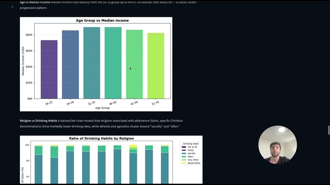
Age vs Median Income Median income rises steadily from the 18–25 group up to the 41–50 bracket, then levels off — a classic career-progression pattern.

Religion vs Drinking Habits A stacked bar chart reveals that religions associated with abstinence (Islam, specific Christian denominations) show markedly lower drinking rates, while atheists and agnostics cluster toward "socially" and "often."

Multivariate — Where Do Patterns Converge?
Full Correlation Heatmap
The complete correlation matrix across all 19 numeric features shows that drinks, smokes, and drugs form a cluster of moderate positive correlations — users who drink heavily are more likely to smoke and use drugs.

Research Questions
Question A — Which combination of 3 lifestyle features produces the largest user groups?
Method: Count the number of users in every unique drinks × smokes × drugs combination. Display as a treemap (rectangle size = group size) and a ranked bar chart.
Plot: Treemap + horizontal bar chart
Finding: A small number of lifestyle combinations account for the majority of users. The dominant group is socially-drinking, non-smoking, non-drug-using users — the "mainstream social" proto-persona. This concentration confirms that the data is not uniform: users genuinely cluster around a few lifestyle profiles.

Verdict: ✅ Supports the persona theory — dominant groups exist.
Question B — Which 3 features contribute so little that removing them won't affect grouping?
Method:
- Coefficient of Variation (CV) bar chart — features with low CV are nearly constant across all users and cannot separate them into groups.
- Correlation heatmap (lower triangle) — features that are highly correlated with another are redundant; removing one loses no information.
Plot: Side-by-side: CV bar chart + correlation heatmap
Finding: Features with the lowest variance are the weakest separators. Any feature that is both low-variance and strongly correlated with another feature is a prime candidate for removal before clustering. This gives a principled, data-driven answer to feature selection.

Verdict: ✅ Identifies 3 removable features — reduces noise before clustering.
Conclusion
The research question is supported by the data.
Four pieces of evidence back the hypothesis that distinct dating personas exist in this dataset:
- Lifestyle habits are correlated — drinks, smokes, and drugs move together, forming a natural habit-cluster axis.
- A few combinations dominate — the treemap shows users concentrate around a small number of lifestyle profiles rather than spreading uniformly.
- Features have high separating power — age, income, and days_since_online show high variance, giving any clustering algorithm meaningful axes to work with.
- Demographic patterns are systematic — the gender income gap and generational smoking patterns confirm that the data has internal structure, not random noise.
The cleaned dataset produced by this notebook is the direct input for the next step: K-Means or hierarchical clustering to formally identify and label the personas.
How to Run This Notebook
- Open in Google Colab
- Run Cell 3 (
!pip install kagglehub) — no API key needed - Run all cells top to bottom
- The cleaned CSV is saved to
/mnt/user-data/outputs/okcupid_cleaned.csv
Dependencies: pandas, numpy, matplotlib, seaborn, scikit-learn, squarify, kagglehub
File Structure
EDA_OKCUPID_personas.ipynb    ← Main notebook
KAGGLE_README.md              ← This file
Benjamin — Data Science Assignment 1, 2026
- Downloads last month
- 74